A labeled dataset for building HVAC systems operating in faulted and fault-free states

The newly expanded dataset contains experimental and simulated data across the seven HVAC systems types and configurations that are represented – the majority being simulated. Diverse facilities and simulation tools were used to create the data, and methods to impose the faults were created for each fault, given the specific HVAC system of focus, the control sequences that defined its operation. These facilities and tools, HVAC system details, and fault methods are described in the following, as is the metadata schema that was applied to the data. Provision of the metadata enables ease of interpretation of the data, and supports users of the dataset who wish to employ more automated procedures to interface FDD algorithm instances with the data.

Facilities and simulation tools

The simulated datasets were created using HVACSIM+ and an EnergyPlus-Modelica co-simulation. HVACSIM + was developed by the US NIST³⁰, the Modelica Buildings Library³¹ is developed by the Lawrence Berkeley National Laboratory, and EnergyPlus³² is developed by several contributors through funding from the US Department of Energy. Described with respect to other modeling tools in³³, HVACSIM+, Modelica, and EnergyPlus are non-proprietary tools to model the behavior of building HVAC systems using physics-based approaches. In addition, Modelon’s air conditioning library was used to model the refrigerant side faults in the RTU system³⁴. This library provides ready-to-use refrigeration cycle templates and a wide range of components to create a variety of air conditioning system configurations.

Four experimental research facilities were used to create data and to develop and validate simulation models:

1. 1.

   FLEXLAB located at the Lawrence Berkeley National Laboratory in Berkeley, California, for the generation of the single-zone CAV data set and the variable-air-volume (VAV) AHU data set⁹.

2. 2.

   The Flexible Research Platform (FRP) located at the Oak Ridge National Laboratory in Oak Ridge Tennessee, for the generation of RTU data sets⁹.

3. 3.

   The Energy Resource Station facility was previously located at the Iowa Energy Center in Ames City, Iowa, for the development and validation of DD-AHU, FCU and FPU simulation models, and for creation of multi-zone VAV AHU data³⁵.

4. 4.

   The RTU facility is located in the Thermal Technology Facility (TTF) at the National Renewable Energy Laboratory in Golden, Colorado, for the validation of the RTU simulation model. NREL’s TTL is a flexible multipurpose laboratory that enables detailed evaluation and development of building and thermal energy systems. The TTF research space reaches 11,000 sq.ft. Two RTUs—a 5-ton/SEER 17 (RTU 1) and a 6-ton/IEER 23 (RTU 2) are installed in the TTL to develop comprehensive performance maps suitable for use with whole-building energy simulation computer programs. The SEER 17 contained a two-stage scroll compressor with R-410A, single-speed condenser fan, direct-drive variable-supply air fan with a high-efficiency motor, low leak dampers, hot gas reheat humidity control, and an economizer. The IEER 23 contained a variable-speed direct-drive compressor, variable-speed fans, and control logic that maintained the compressor and thermal expansion valve (TXV) within their performance limitations³⁶.

Field data representing faulted and un-faulted rooftop unit operation is also included in the dataset. This data was collected from two RTUs, one in a restaurant building in Milford, CT and another one in a distribution center building in Colchester, CT. Table 1 summarizes these sites and the RTUs.

System configurations and control sequences

The configurations and sequences for each system in the data set are comprehensively documented for users of the data in an inventory file. This information is often needed to specify controls-specific parameters in fault detection and diagnostic algorithms. To illustrate the form and content of this information, two examples are presented – the fan coil unit system, and the boiler plant.

Fan coil unit

Figure 1 contains the schematic representation of the fan coil unit (FCU) system.

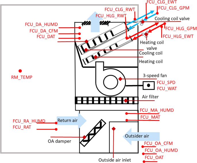
Schematic diagram of the FCU.

The FCU is scheduled for automatic operation on a time of day basis for occupied and unoccupied mode.

Occupied mode (Monday – Friday 6:00AM–17:59PM)

During these hours, the system is in Operate Mode. Five control sequences – control, outdoor air damper control, cooling coil valve control, heating coil valve control sequence, and zone temperature setpoints – were set during the simulation.

• Fan control

• OA damper control

• Cooling coil valve control sequence

  • The PID control is used to adjust the cooling coil valve position. The setpoint dead band is 1 °F. If the actual room temperature is beyond 1 °F of the cooling setpoint, the FCU is in the “cooling” mode, and the cooling coil valve PID loop is enabled and the cooling valve position will be controlled by the cooling coil valve controller PID output. When the room temperature falls below 1 °F compared to the cooling setpoint, the cooling PID is disabled and the valve fully closed.

• Heating coil valve control sequence

  • The PID control is used to adjust the heating coil valve position. The setpoint dead band is 1 °F. If the actual room temperature is beyond 1 °F of the heating setpoint, the FCU is in the “heating” mode, and the heating coil valve PID loop is enabled and the heating valve position will be controlled by the heating coil valve controller PID output. When the room temperature falls below 1 °F compared to the heating setpoint, the heating PID is disabled and the valve fully closed.

• Zone temperature setpoints

• Shutdown mode

  • The shutdown mode is only triggered by the low temperature protection described below. Under the shutdown mode, the fan is constantly off, and the OA damper is fully closed.

• Low Temperature Protection

  • During the simulation, when the mixed air temperature is below 35 °F and persists for 300 seconds, the FCU system will switch to the shutdown mode to prevent freezing the coil. The shutdown mode will last until the end of the day. The system will be turned back to normal operation at the beginning of the next day.

Unoccupied mode

During these hours, the system is in Setback Mode. The operation is similar to the operation mode except two additional settings as:

Boiler plant

Figure 2 illustrates the configuration of the boiler plant system. This system has two identical boilers and two hot water pumps and provides hot water to heating coils in the air-side system.

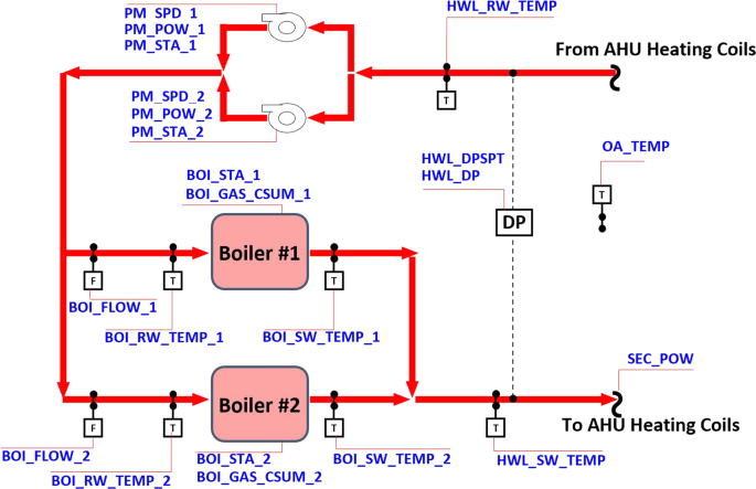
Schematic of the studied boiler plant system.

The boiler plant system is controlled by two supervisory controllers and two local controllers (Table 2). One supervisory controller determines the number of the operating boilers using a state machine and the calculated heat load, as shown in Fig. 3. The heating load is calculated from:

where \({\mathop{v}\limits^{^\circ }}_{hw}\) is the volumetric flow rate of the hot water, \({T}_{hw}^{ent}\) and \({T}_{hw}^{lea}\) are the temperature of the hot water entering and leaving the boiler plant system, respectively. The other supervisory controller determines the number of operating hot water pumps, as shown in Fig. 4.

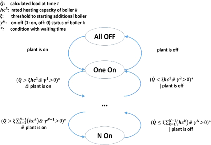
Staging control of boilers (ξ = 0.95 and waiting time: 30 min).

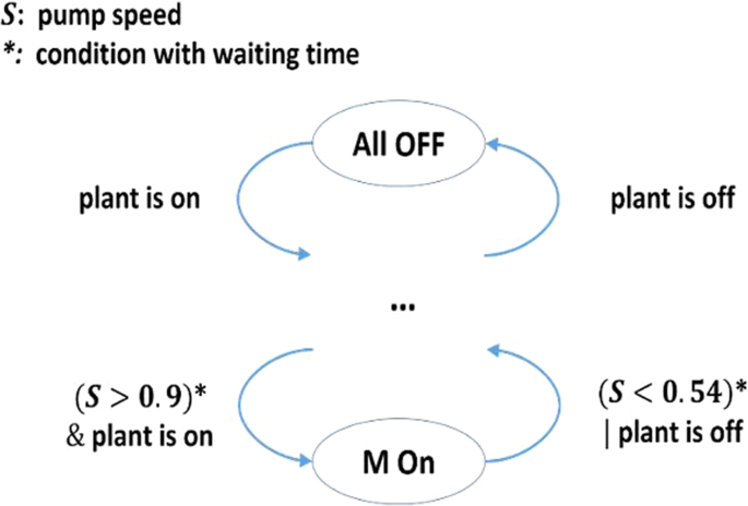
Staging control of hot water pumps in the boiler plant system (waiting time: 30 min).

Fault scenarios and methods of fault imposition

Tables 3–10 summarize fault profiles and how each fault was imposed for each of the systems and fault scenarios. For the simulated datasets, each fault type and intensity were imposed for a full calendar year of operation – the exception being the simulated RTU dataset that covered a 100-day cooling season. For the experimental and field test datasets, fault type-intensity combinations were captured for one to 183 days of operation.

The RTU dataset that was acquired from field measurements reflected a naturally occurring compressor staging fault and a refrigerant undercharging fault.

Method of Brick schema model development

The Brick schema²⁹ offers classes and subclasses, of which the equipment class was used to designate the HVAC system components represented in the fault dataset. Similarly, the point subclass was used to design sensor measurement and control system data points. In addition, the schema offers ‘relationships’, of which hasPart, hasPoint, and feeds, are relevant to describing the fault dataset. Figure 5 illustrates the 5-step process that was used to generate the Brick models for each HVAC system in the dataset. Among them, Step 4 is automated while the other steps are performed manually.

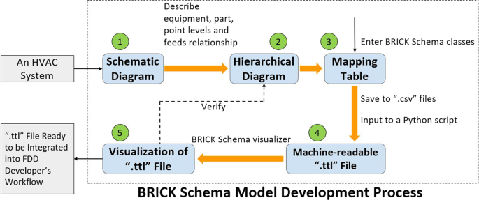
Flow of the Brick Schema model development.

Step 1: Conceptualization of Brick relationships using mechanical drawing or schematic

The schematic representations for each system were reviewed to identify the major components for the overall system, to develop compositional (“hasPart”) relationships. For each major component, we identify all of the associated sensor/control points to develop “hasPoint” relationships. Lastly, we identify the order in which the given media (air, water, etc.) flow through the system to develop sequential (“feeds”) relationships between different equipment.

Step 2: Creation of hierarchical diagram to visualize Brick relationships

After identifying the components and sensor/control points of the system in Step 1, we indicate which equipment has which components (“hasPart”), which equipment or component has which sensor and control data points (“hasPoint”), and which equipment feeds into another equipment (“feeds”).

Step 3: Mapping system components to Brick classes

All equipment, components, and sensor/control data points in the hierarchical diagram are mapped to a Brick schema class and tabulated. The equipment and the sub components are mapped to a subclass of the Brick “equipment” class (e.g., chiller, AHU, and RTU) and the sensors and the control points will be assigned a type subclass of Brick “point”.

For each row (i.e., each component), we designate the relevant relationships, other components it connected to and these components. This way, we are able to incorporate all the components, their types and how they are related to other components.

Step 4: Execution of script to create a .ttl file

The tables generated in Step 3 are exported as CSV files and imported to a Python script that generates a Brick model in the form of a machine-readable .ttl file. The script iterates through each row of the table, assigning all components and points to a specific instantiation of a Brick class and corresponding relationships. The .ttl file can be accessed by an FDD algorithm (or other applications), enabling more efficient and standardized retrieval of system metadata using SPARQL queries. This streamlines the interpretation of data semantics within the FDD or other applications.

Step 5: Visualization of the Brick model to validate accuracy

The generated Brick model is verified by visualizing it and comparing it to the hierarchical diagram in Step 2. We used Brick Studio for the visualization and ensured that all the components in the data sets were present and the relationships between them were labeled correctly.