Tests for associations between sexual dimorphism and patterns of quantitative genetic variation in the water strider, Aquarius remigis

Study animal

Aquarius remigis are surface-dwelling semiaquatic bugs (Hemiptera, Gerridae), commonly called water striders, found on streams and small rivers across much of sub-arctic North America (Preziosi and Fairbairn 1992). Adults are primarily wingless (>99% in most populations), and following the precedent of previous studies of the genetics of body size variation in this species (Preziosi and Roff 1998; Fairbairn 2007), our analysis includes only wingless individuals.

Females average 5–11% longer than males, but the magnitude and direction of sexual dimorphism varies greatly among body components (Table 1 and Supplementary Figs. S2 and S3). This reflects the underlying pattern of sexually antagonistic selection: fecundity selection favors longer abdomens in females whereas sexual selection favors longer genitalia in males (Preziosi et al. 1996; Preziosi and Fairbairn 1996, 1997, 2000; Ferguson and Fairbairn 2000; Sih et al. 2002; Bertin and Fairbairn 2005).

Sex is determined chromosomally in A. remigis, with females having two X chromosomes, and males one (Fairbairn et al. 2016). The absence of a Y chromosome simplifies the quantitative genetic analyses and interpretation of sex-linked effects because all sex-linkage can be ascribed to X-linked effects. In addition, the potential for X-linked effects is high because the X chromosome is the largest chromosome in the karyotype, averaging 13% larger than the largest of the 10 autosomes and comprising 14% of the haploid chromosome complement (Fairbairn et al. 2016).

Previous studies of the additive genetic (co)variance structure of morphological traits in A. remigis established that the lengths of the somatic and genital components have significant heritabilities and inter-sex additive genetic correlations (Preziosi and Roff 1998; Fairbairn 2007). In addition, full-sib estimates of r_A showed the predicted negative correlation with the magnitude of dimorphism for a suite of 5 independent size traits (Fairbairn 2007). The study described herein greatly extends this work by increasing the number of traits included and by providing estimates of autosomal additive, autosomal dominance and sex-linked (co)variances.

Analysis of the genetic architecture of sexual dimorphism

The majority of experimental designs or analyses of unmanipulated populations cannot estimate both autosomal dominance and additive X-linked variances and the former are typically assumed to be zero and omitted from the analysis (see “Dominance and maternal variances” in Supplementary Information and Supplementary Table S1). Maternal effects are also frequently omitted. This can be justified because maternal effects are most frequently found during juvenile or larval stages and are greatly reduced or absent in adults (see Supplementary Fig. S4 and associated references).

Our analysis uses the animal model (Lynch and Walsh 1998) based on a pedigree from a three-generation, double-first cousin breeding design developed specifically to estimate the autosomal additive and X-linked additive variances (Fig. 1; Fairbairn and Roff 2006). Simulations have shown that, when analyzed using the animal model approach, this design produces more precise and unbiased estimates of sex-specific additive (co)variances than alternate approaches such as mean squares (Meyer 2008). This analysis also estimates the sum of dominance and maternal variances but cannot adequately estimate each separately (Meyer 2008). As noted above, maternal effects are often absent in adults and on average account for a much lower proportion of phenotypic variance than do dominance effects: 3% (Supplementary Fig. S1) versus 14% (Wolak and Keller 2014). Given the potentially small contribution of maternal effects relative to dominance, we ascribe the dominance + maternal genetic variance component to dominance variance.

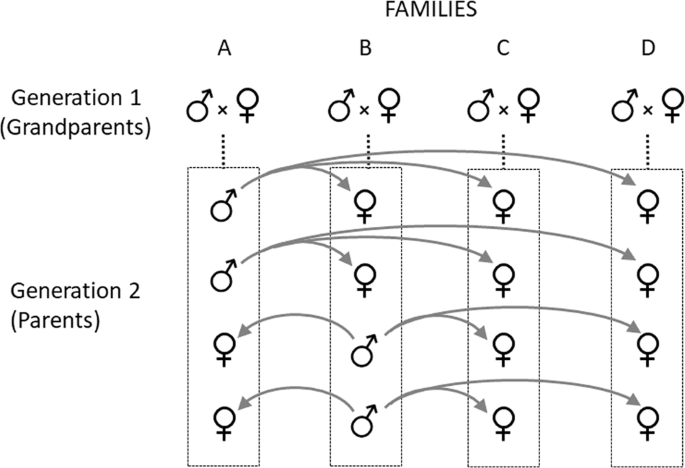
Each three-generational breeding unit includes four unrelated grandparental pairs (grandparental generation), plus four of their full-sib offspring (parental generation) with sex ratios as indicated, plus the offspring (F1 generation) of a prescribed set of matings among the families in generation 2. To produce the F1 generation (not shown), four sibs from each family are crossed as indicated by the gray arrows. Brothers from family A mate with sisters from families B, C and D. Similarly, brothers from family B mate with sisters from families A, C and D. This design produces a gradation of relationships in the F1 generation including full sibs, half sibs, first cousins and double-first cousins.

Experimental protocols

The experiment was conducted in three consecutive, independent replicates (Table 2). Each replicate was initiated using eggs collected from laboratory-acclimated adults collected from Rattlesnake Creek, in Santa Barbara County, California. Individuals reared from these eggs formed the GP generation. Stratified random sampling and randomized blocked rearing protocols were used to minimize the possibility that environmental effects could bias our estimates, and all rearing was done in environmental chambers set at 25 °C, under a light regime of 14hL:10hD. Adults were preserved in 70% ethanol for later photographing and measurement. Detailed descriptions of the founding samples (Supplementary Table S2), rearing regimes and experimental protocols are given in the Supplementary Information. The final data included individuals contributing to 36 breeding units plus additional full-sib families from the GP and P generations (Table 2).

Traits and measurement protocols

All traits (Table 1) are linear measures taken in ventral view, and none are linear components of any other. Photographs of males and females showing the somatic and genital measurements are shown in Supplementary Figs. S2 and S3 (see also Fairbairn 2005, 2007, 2016; Fairbairn et al. 2003). Somatic measurements include the lengths of the head, thorax, abdomen and femora of the front, middle and hind legs, plus the width of the abdomen and the width of the front femur at its widest point. Two additional somatic measurements capture sex-specific morphologies characterizing the last abdominal segment, segment 7. This segment is elongated in males to facilitate clasping females, and the shape of the distal ventral margin is modified to facilitate movement of the phallus (Fairbairn et al. 2003). In addition, the lateral margins extend backward to form a pair of connexival spines that flank the genital segments and, in some species, aid females in repelling male mating attempts (Arnqvist and Rowe 2002). To characterize size dimorphism in segment 7, we measured the length of the outer (lateral) margin of segment 7 and the distance between the tips of the connexival spines.

As in other gerrids (Rowe and Arnqvist 2012), the genitalia of A. remigis have evolved through sex-specific modifications of the three terminal segments of the primitive abdomen (segments 8, 9 and 10) (Fairbairn et al. 2003). To capture sexual differences in genital size for homologous genital components, we measured the length of segment 8 and the combined length of segments 9 and 10.

All measurements were taken under a dissecting microscope, following standard protocols established in previous studies (e.g., Preziosi and Fairbairn 1996, 1997; Bertin and Fairbairn 2007). A detailed description can be found in Supplementary Information.

Our questions pertain to the magnitude of sexual dimorphism, without regard for which sex is larger. To quantify this, we used the following index: (size of the larger sex divided by size of the smaller sex) – 1, which has the conceptual advantage of being zero for monomorphic traits. This is the absolute value of the dimorphism index (SDI) of Lovich and Gibbons (1992), which is arbitrarily assigned to be negative if males are the larger sex. Hence, our index is abs(SDI).

For the analysis of genetic variance structure, we standardized the data for each trait across the entire data set, including both sexes and all generations and replicates, by subtracting the mean and dividing by the standard deviation. This has the effect of removing any possible confounding influence of differences among traits in means and phenotypic variances.

Estimation of (co)variances

We partitioned phenotypic (co)variances for each sex into autosomal additive and autosomal dominance (co)variances and sex-linked additive variance using quantitative genetic linear mixed models, commonly known as ‘animal models’ (Lynch and Walsh 1998), as proposed by Fairbairn and Roff (2006) and implemented in the asreml-r software package. Matrix inverses for each genetic relatedness matrix, required to estimate genetic (co)variances, were formed using the nadiv (Wolak 2012, 2013) package for R. Models that included sex-linked dominance variance failed to converge, but the models did converge when sex-linked dominance was omitted from the estimation. The experimental procedure is, in principle, capable of estimating this variance component (Meyer 2008), indicating that the failure to converge was most likely due to the sex-linked dominance being too small to estimate. In such cases, the algorithm tends to become unstable and may not be able to converge. We therefore excluded this variance component from our final models.

The inverse of the Average Information matrix was used to obtain approximate standard errors for (co)variances from the model and, in conjunction with the delta method (Lynch and Walsh 1998, Appendix 1), to obtain approximate standard errors on linear functions of the model estimated (co)variances (e.g., variances expressed as proportions of phenotypic variance and correlations).

Genetic independence of traits

To determine if all of the traits can legitimately be considered as different traits at the genetic level, we did an initial analysis of pairwise genetic correlations among traits within each sex (Supplementary Tables S3 and S4). All were significantly less than 1.0, and almost a third (43 of 132) did not differ significantly from 0. All of the significant correlations were positive but the magnitudes averaged only 0.47 in males and 0.32 in females, and only 5 exceeded 0.8. These correlations show that there is adequate scope for separate evolution of the traits and therefore we retained all 12 traits in our analyses.

Independence of estimates of abs(SDI)

Because all traits are morphological traits, it is likely that they are phenotypically correlated within individuals, thus possibly making estimates of SDI not statistically independent. To eliminate this possibility, we randomly assigned individuals to one of 12 equal-sized subsets and estimated mean values for only one trait per subset (thus a subset for head width, another for thorax, etc.). Our estimates of abs(SDI) for each trait are derived from these subsets and so the estimates for the 12 traits are statistically independent. The reported results are based on these values. (We also did the analysis using the trait values from the undivided data set and this did not change any of our conclusions.)

Model validation

We began our estimation of genetic (co)variances with a preliminary analysis of each sex separately, incorporating generation and replicate as fixed effects and the additive, dominance and sex-linked variance components as random effects. Model convergence was obtained for all 12 traits for both sexes. However, the sex-linked additive genetic variance in males, calculated as a proportion of the total phenotypic variance, averaged only 0.34% compared to 9.91% in females. The very low value in males suggested that the sex-linked additive covariance was probably insignificant or very small. To test this, we ran the full model in which males and females were incorporated into a single model but treated separately by considering them as separate environments, as suggested by Falconer (1952):

where V_pM, V_pF are the phenotypic (p) variances of the males (M) and females (F), respectively, and \(Cov_{pMF}\) is the phenotypic covariance between the sexes. The phenotypic covariance matrix is decomposed into autosomal additive (a) and dominance (d), sex-linked additive (x), and environmental (e) components, where the cross-sex residual covariance is fixed to zero because this parameter is not estimable when traits are only ever expressed in separate female or male environments (Wolak et al. 2015).

Convergence was obtained for only three traits and in all of these the sex-linked additive covariance between the sexes was not statistically different from zero. Therefore, all the models presented in this paper assume a sex-linked additive genetic correlation between the sexes of zero, i.e. \(Cov_{xMF} = 0\).

An important consequence of the very small sex-linked genetic variance in males is that the type of dosage compensation, if any, should not matter. We ran the analyses using a no-dosage compensation model (“ngdc” option in R package nadiv; Wolak 2012, 2013) and a full dosage compensation model (“hedo” option in nadiv). As expected, differences between estimates of male sex-linked genetic variance were less than 10⁻⁸. The results for the variance components as proportions of the total phenotypic variance were identical (i.e., independent of the dosage compensation model used) and thus we report only one set of values.

The usual statistical analysis of linear regression is potentially biased by collinearity, the influence of outliers, excessive leverage and covariance among predictor variables. These factors are hard to evaluate with just 12 data points. To circumvent such problems, we adopted a randomization approach (Roff 2006). The general procedure was as follows: first, we ran the usual linear regression analysis and stored the F value, which we designate as F_obs. Next, we randomized the abs(SDI) estimates and reran the regression analysis, storing the F value as F₁. This randomized procedure was repeated 10,000 times. The null hypothesis of no covariation was tested by computing the number of times the F value from the randomized data set exceeded F_obs, which we denote as \(N_{F_i > F_{obs}}\). Probability was estimated in the usual fashion for a randomized protocol as \(P_r = \left( {N_{F_i > F_{obs}} + 1} \right)/10,001\), where the extra 1 represents the observed F value. For a one-tailed test the randomization approach was modified in that to be included in \(N_{F_i > F_{obs}}\) the slope of the regression must also be in the predicted direction. For comparison, we provide the regression estimates for the regression using the observed data set, the associated probability, P_obs, and the probability from the randomization method, P_r.

The full genetic model described above (i.e., additive, dominance and sex-linked variance components) was compared to the constants-only model (i.e., with no genetic effects) using the log-likelihood ratio test (Wilson et al. 2010). Convergence was obtained for all morphological traits and in all cases the full model accounted for significantly more variance than the constants-only model and this difference was highly significant (P < 10⁻⁶).